Every reporting cycle produces a slide with a single number on it: average handling time, median deal size, mean cost per unit. The number is correct, easy to read, and hides almost everything a decision-maker needs to know. Two teams can post the same average and operate nothing alike. One runs steady, the other swings between finishing in an hour and losing three days to a stuck ticket. An average cannot tell those two apart, and neither can the bar chart that usually carries it.
The box plot chart exists for that gap. It compresses a full set of observations into a shape that shows where the middle sits, how far the values spread, whether they lean high or low, and which points sit far enough out to deserve a name. It is one of the few chart formats that answers a question about consistency rather than size, and consistency is what operations, quality, hiring, and pricing conversations tend to turn on.
What follows covers the parts of a box plot, how to read an unfamiliar one, the reporting jobs it handles well, the information it discards, how to build it in PowerPoint and Google Slides, how it compares with other distribution charts, and the mistakes that get it challenged in a meeting.
The Problem the Average Hides
Take two support teams reporting ticket resolution time for the same quarter. Both post an average of 6.2 hours. On a bar chart, the two columns are the same height and the review moves on.
The five-number summaries tell a different story. Team A runs from a fastest ticket of 1.5 hours to a slowest of 11, with the middle half of its work landing between 4.8 and 7.5 hours and a median of 6.0. Team B has a median of 3.4 hours, faster than Team A on most days, with the middle half falling between 2.1 and 7.9. Team B also has a handful of tickets that ran past 24 hours, and those few cases drag its average up to match a team that never has a bad day.
Put side by side as box plots, the difference is visible before anyone reads a label. Team A shows a narrow box sitting high; Team B a wider box sitting lower with points scattered above the whisker. Team A has a speed problem worth investigating. Team B has an escalation problem, and fixing the tail would improve its reported average more than anything done to routine tickets.
That is the entire argument for the format. A strong data presentation shows the shape of the evidence rather than a summary that flattens it, and the box plot does that in less space than any alternative.
What Makes a Box Plot Chart
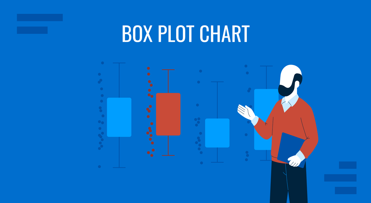
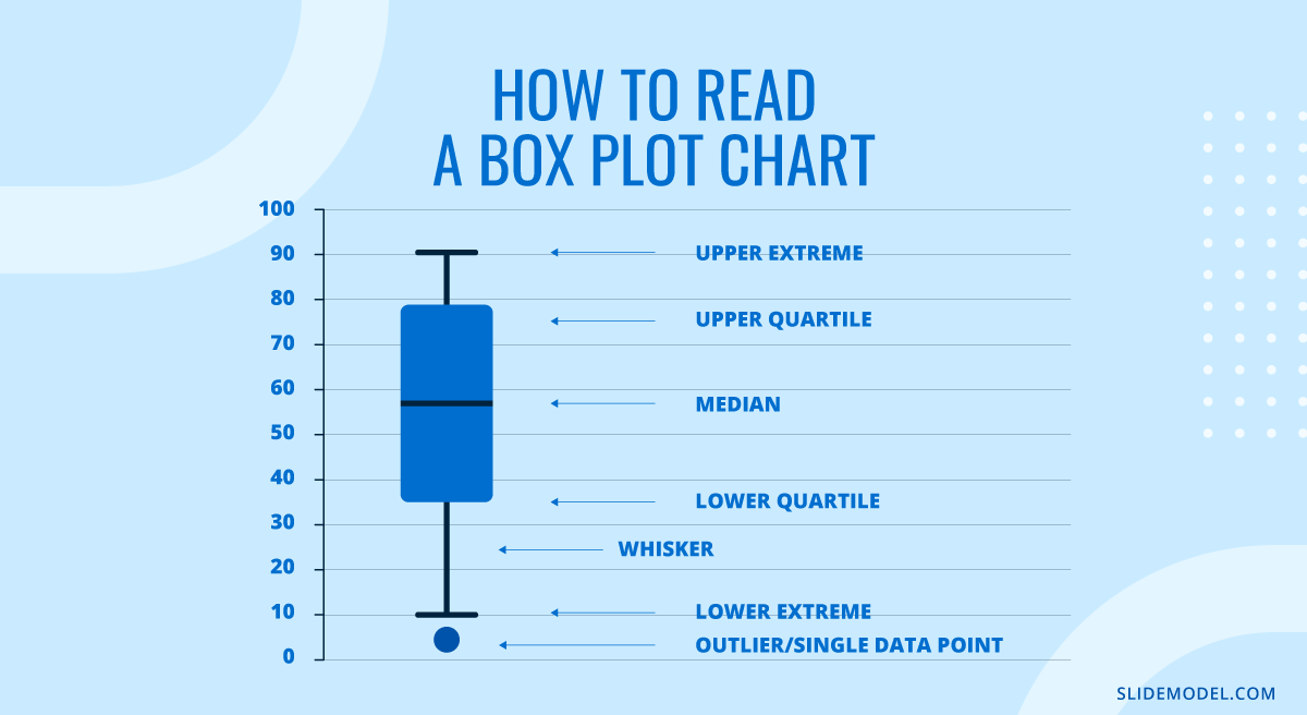
A box plot chart, also called a box-and-whisker plot, draws a five-number summary of a numeric variable along a single axis. Each mark corresponds to a specific order statistic, which is why the format translates well across tools and audiences.
The Five Numbers
The median is the line inside the box. Half the observations sit above it and half below. It is not the mean, and on skewed data, the two can sit far apart.
The first quartile forms the lower edge of the box, with a quarter of the values below it. The third quartile forms the upper edge, with a quarter of the values above it.
The interquartile range, the distance between those edges, is the box’s width. It contains the middle 50% of the data, making box width the fastest available read on consistency.
The whiskers extend toward the extremes, stopping at the farthest observation still within a defined limit. Anything past that limit is drawn as an individual point.
Because these are rank-based figures, they don’t move much when a single extreme value changes. Replace one observation with a number ten times larger and the mean shifts immediately, while the median and quartiles usually do not move at all. That resistance is why the format is trusted in quality and process work, where the occasional wild reading is expected rather than surprising.
Why the Whiskers Stop Where They Do
The common convention draws whiskers out to the furthest observation within 1.5 times the interquartile range of the nearest box edge. The 1.5 is a judgment call rather than a derived constant, but it has a rationale. Under a normal distribution, the quartiles sit roughly 0.67 standard deviations from the center, which puts those fences at about 2.7 standard deviations out. Around 0.7% of a normal sample falls beyond them, or seven observations in a thousand.
That threshold suits business data. It is loose enough that a clean process produces almost no flagged points, and tight enough that genuine irregularities surface. It also explains a recurring confusion in large datasets: with 10,000 observations, a perfectly well-behaved process still produces around 70 points outside the fences. They are not defects. They are what a distribution does when you sample it enough times.
Not every tool uses the same rule. Some draw whiskers to the absolute minimum and maximum, removing outlier marks entirely, and others stop at the 5th and 95th percentiles. State the convention in a footnote whenever an audience will act on the chart.
Where the Format Came From
The design is older than most people assume. Mary Eleanor Spear published a range bar in her 1952 book Charting Statistics that already used a box for the interquartile range with lines extending to the extremes, twenty-five years before John Tukey formalized the box-and-whisker plot in Exploratory Data Analysis. Tukey added the outlier fences and the vocabulary that stuck.
A 1978 paper in The American Statistician by Robert McGill, John Tukey and Wayne Larsen added two variations still worth knowing. Variable-width boxes scale each box by sample size, so a group built on 40 observations does not visually outweigh one built on 4,000. Notched boxes add a pinch around the median, approximating a 95% confidence interval, calculated as roughly 1.58 times the interquartile range divided by the square root of the sample size. When the notches of two boxes don’t overlap, the difference between those medians is unlikely to be noise, turning a descriptive chart into something closer to a statistical test.
Reading an Unfamiliar Box Plot in Four Passes
Most people freeze in front of a box plot because they try to absorb it at once. Reading it in a fixed order takes about forty seconds and produces a usable interpretation every time.
First, find the median lines and compare them across groups. This answers the typical case question. Which group is faster, cheaper, higher paid, more productive on an ordinary day? Ignore everything else until this is settled.
Second, compare box sizes. A short box means the middle half clusters tightly, so the process is predictable and the median is a fair summary. A tall box means half the observations are already scattered before you reach the extremes, and any single-number summary of that group will mislead.
Third, check whisker symmetry. An upper whisker noticeably longer than the lower one means right-skewed data, the normal state of durations, costs, and deal values. A long lower whisker on that kind of measure is unusual and usually points to a data problem or a different subgroup mixed into the sample.
Fourth, look at the individual points. Their count matters as much as their position. One isolated point far out is an event with a story attached. A cluster of points along the same edge is a second population folded into the group by accident, such as enterprise accounts sitting inside a chart about self-serve customers.
Run those four passes on each group, and the comparison writes itself. The habit also makes it harder to be talked into a conclusion the chart does not support, which is a reasonable definition of chart literacy for anyone who reviews key metrics regularly.
Where Box Plots Earn Their Place in Business Reporting
The format fits a specific class of question: how does the same measurement behave across several groups, when the variation matters as much as the middle.
Service and cycle times are the natural home. Ticket resolution, order fulfillment, invoice approval, hiring stage duration, and call handling all produce right-skewed distributions where the average is inflated by a tail nobody wants to discuss. A box plot per team, region, or quarter puts that tail on the slide instead of leaving it inside a mean.
Compensation and pay equity reviews use the format almost by default. A box plot per job level shows band overlap, where each band’s middle sits against where policy says it should, and which individuals fall outside their band. Because it shows quartiles rather than individual salaries, you can present it widely without exposing anyone.
Process quality and supplier comparison work the same way. Fill weights, tolerances, defect counts, and delivery variance across suppliers are questions about consistency first and level second, and box plots rank candidates on both at once. That fits the variance thinking behind data-driven decision making, where the decision hinges on risk as much as on the headline figure.
Experiment and survey results benefit when the distribution does something the average conceals. Ratings that split into a satisfied group and a frustrated one, or before-and-after comparisons where the spread narrows while the median barely moves, are cases where the box carries the real story. When presenting survey results to a mixed audience, a box plot beside a simple average often prevents later arguments.
What the Box Throws Away
A box plot is a summary, and every summary discards something. Being explicit about what you lose separates a defensible chart from a decorative one.
The largest blind spot is shape within the box. A box plot cannot distinguish a single tight cluster of values from two separate clusters sitting either side of the median, since both produce the same rectangle. This matters more than it sounds, because business measurements are usually mixtures of processes. Support tickets split between password resets and integration failures. Deal sizes split between renewals and new logos. A box plot of the combined population describes a middle that no actual case occupies.
Sample size is the second loss. A standard box plot looks identical whether it summarises 12 observations or 12,000, and quartiles estimated from a dozen points are not stable enough to compare. Variable-width or notched boxes solve this, and so does annotating each group with its sample count.
Large samples create the opposite problem. Heike Hofmann, Karen Kafadar, and Hadley Wickham addressed it with the letter-value plot, published in the Journal of Computational and Graphical Statistics in 2017, which replaces the single box with nested boxes covering 50%, 75%, 87.5% of the data and beyond. It shows tail structure that a standard box plot reduces to a smear of dots, and for datasets in the tens of thousands, it is the better instrument.
Building a Box Plot Chart for a Presentation
The build is short. The decisions inside it are where charts go wrong.
In PowerPoint and Excel
PowerPoint has had a native box plot since the 2016 release. Go to Insert, then Chart, then the Statistics category, and choose Box and Whisker. PowerPoint opens a small worksheet where each column is one group and each row is a single observation, not a summary. This trips people up constantly. Do not paste in quartiles you calculated yourself; paste the raw values and let the chart derive the five-number summary.
With the chart placed, right-click the boxes and open Format Data Series. Four settings there change what the chart communicates. Show inner points plots every non-outlier observation alongside the box, worth turning on for groups under about 50 cases. Show outlier points controls the marks beyond the whiskers and should stay on in nearly all cases. Show mean markers adds a cross at the arithmetic mean, and the gap between that cross and the median line is often the most persuasive detail on the chart. Show mean line connects means across groups and is usually clutter.
The same pane holds Quartile Calculation, with a choice between inclusive and exclusive median. Exclusive is the Excel default and matches QUARTILE.EXC; inclusive matches QUARTILE.INC and the method taught in most statistics courses. The two produce visibly different boxes on small samples, so if your chart has to reconcile with a figure someone else calculated, match their method before the meeting rather than during it. When the numbers live in a workbook, keeping the link intact while moving Excel data into slides saves a rebuild on every refresh.
In Google Slides
Google Slides has no box plot type, and neither does Google Sheets. The usual workaround builds a candlestick chart from four calculated columns using MIN, QUARTILE(range,1), QUARTILE(range,3), and MAX, then inserts it through the chart editor. The result looks like a box with whiskers and works for simple comparisons, but it cannot show a median line or mark outliers, which removes two of the format’s intended uses. For anything analytical, build the chart in Excel and place it as an image, or use a shape-based template. The general workflow for making a graph in Google Slides applies once the chart exists.
The Box Plot Against Other Distribution Charts
Choosing between distribution formats depends on how many groups you are comparing and how much shape detail the audience needs.
A histogram shows the full shape of one distribution, including any second peak a box plot would flatten. The cost is that histograms do not stack: three histograms side by side are three separate reads, while three boxes are one. Use a histogram when a single distribution deserves its own slide, and a box plot when the comparison is the point. Building a histogram in PowerPoint follows the same Insert > Chart > Statistic route.
A violin plot mirrors a smoothed density curve on both sides of the axis, exposing bimodality that defeats a box plot, and it handles many groups better than histograms. The drawback is interpretive: violin width depends on a smoothing parameter most viewers do not know exists, and executive audiences rarely have a reference for the shape. A violin with a small box inside it is the usual compromise for analytical readers.
A strip plot or jittered dot plot shows every observation as a point, making it the most honest option for groups with roughly 50 cases or fewer. Above a few hundred points, it turns into a solid block. Overlaying points on a box plot, which is what Show inner points does, gets most of the benefit at small sample sizes.
A bar chart with error bars is the format box plots most often replace. Error bars usually show standard deviation or standard error, which assume a symmetric distribution and say nothing about skew or outliers. On right-skewed data, which most operational data is, the error bar understates the upside risk. There are cases where error bars remain the right call, mostly when the audience expects a mean with a confidence interval, but the choice should be deliberate.
A column chart of averages is the weakest option for this purpose and by far the most common. It shows one number per group and implies a precision the data doesn’t support. If a slide currently carries average handling time per team as columns, swapping to box plots usually changes the conversation in the room.
Visuals That Work Alongside a Box Plot
A box plot answers a distribution question and nothing else, so it generally needs a companion.
A time series line covers what a box plot lacks on the axis. Box plots per quarter show how spread changed across four snapshots, while a line chart of the median across every month shows the path between them. The pair reads well as a two-panel slide, with the line establishing direction and the boxes explaining consistency.
A Pareto chart works after a box plot has flagged a tail. Once the audience accepts that a small number of cases distorts the average, a Pareto chart of the reasons behind those cases moves the discussion from diagnosis to action inside the same slide sequence.
A small table of counts and medians under the chart answers the two questions a box plot always raises: how many observations sit behind each box, and what the exact median is. Three columns and a handful of rows absorb most of the objections a skeptical reviewer raises. When the chart has to live in a recurring report, the dashboard layout sets the constraint, and box plots survive downsizing better than most chart types because their meaning sits in position rather than in fine detail.
Where Box Plots Go Wrong
Most failures are recognizable by what the audience does when the slide appears.
The room goes quiet, and nobody asks anything. The format was unfamiliar, and the chart carried no orientation. A one-line caption stating that the box holds the middle half of the data and the dots are individual cases fixes it. Presenters skip that line because the explanation feels basic to them; it is not basic to a finance director seeing the shape for the first time.
Someone asks how many cases are in each group. The chart omitted sample sizes. Box plots drawn from small groups look exactly as authoritative as ones drawn from large groups, and reviewers are right to be suspicious. Annotate each box with its count.
Someone challenges the outliers as errors. The points beyond the whiskers were left unlabelled, so they read as data quality problems. Label the two or three that matter with what they actually were, and the same marks become the most valuable content on the slide.
Two versions of the same chart disagree. Different quartile methods, or one tool drawing whiskers to the extremes while another uses the 1.5 rule. Fix the convention across the reporting pack and state it in a footnote.
The chart is used for part-to-whole data. Market share by segment, budget allocation, and survey response percentages are not distributions of a measurement, and a box plot of them is meaningless. The format needs many observations of one numeric variable per group.
Groups are ordered alphabetically. Sorting by median or box width turns the chart into a ranking readable at a glance, and alphabetical ordering wastes the format’s strongest advantage.
Color carries the only distinction between groups. Fine on a monitor, unreadable when projected badly or viewed by someone with a color vision deficiency. Direct labels under each box and varied fill patterns keep the chart usable, which is the baseline for accessible slides.
FAQs
When is a box plot the wrong choice for a business slide?
When the audience needs exact values, when the data is categorical or part-to-whole, when there is only one group and no comparison to make, or when the sample is small enough that showing every point is both possible and more convincing.
How many groups can one box plot chart hold?
Twelve to fifteen boxes stay readable in a presentation, and beyond that the labels collapse. If the comparison needs more, split it across two charts or aggregate the smallest groups into a combined category with its count noted.
What is the minimum sample size for a meaningful box plot?
Around 20 observations per group is a reasonable floor for the quartiles to mean anything. Below that, plot the individual points instead. Between 20 and 50, plot the box with the points overlaid.
Does PowerPoint create box plots natively?
Yes, since the 2016 release, through Insert > Chart > Statistic > Box and Whisker. The chart takes raw observations rather than pre-calculated quartiles, and the formatting pane controls outliers, inner points, and mean markers.
Why do two tools show different boxes for the same data?
Almost always the quartile method. Inclusive and exclusive median calculations place the box edges differently, and the gap is widest on small samples. Whisker conventions differ too, with some tools reaching to the true minimum and maximum rather than to the 1.5 IQR fences.
Should the mean be displayed alongside the median?
Often yes. The distance between the mean marker and the median line directly measures skew, and it is the fastest way to show an audience why the average they have been reading is misleading.
What does it mean when the median line sits off-center in the box?
The distribution is skewed within its middle half. A median close to the lower edge means values bunch at the low end and thin out upward, which is the usual pattern for durations and costs.
Are points beyond the whiskers always errors?
No. Under the standard rule, a well-behaved process still produces about seven flagged points per thousand observations, so large datasets will always show some. Treat them as cases to investigate rather than defects to remove, and never delete them silently.
How do I introduce the format to an audience that has never seen it?
Show one box with four labels on its first appearance, then drop the labels for the rest of the deck. Describing the box as the range for a typical case and the dots as exceptions is usually enough for a decision-making audience.
What single change improves most box plots on business slides?
Sorting the groups by median and annotating the two or three extreme points with what they were. The first turns the chart into a ranking; the second turns statistical marks into evidence people can act on.
Final Words
A box plot chart is a narrow instrument with a clear job. It compares the distribution of one numeric measure across several groups, and it does that in less space and with less audience effort than any competing format. It will not tell you the shape inside the box; it will not carry a total, and it will not survive an audience that has never had it explained. Those limits are worth accepting when the question on the table is whether a process is consistent, whether two groups genuinely differ, or whether a tail has quietly inflated an average.
The build takes ten minutes. The judgment is in what surrounds it: sample sizes on the boxes, a stated quartile convention, sorted groups, and a label on the outliers that matter. Get those right, and the chart stops being a statistics exercise and becomes the slide that changes what the room decides to do next.